Introduction
Large language models are currently all the rage when it comes to text classification. However, a recent research paper offers an interesting non-parametric alternative. The proposed method is elegant in its simplicity: it combines a text compressor, gzip, with a k-nearest-neighbour classifier. This approach requires no training parameters, making it a lightweight and universally adaptable solution.
The cornerstone of this method lies in two key ideas: first, compressors are good at capturing regularities in data, and second, data points from the same category share more regularity than those from different categories.
In this article, we explore this approach to text classification, discussing its rationale, how it works, and its practical implementation in Python.
The Mechanics of Compression and Classification
The technique proposed in the paper uses combination of a text compressor and a k-nearest-neighbor classifier. But what makes this a viable method for text classification?
At the heart of this approach is the idea that data compressors, like gzip, are skilled at capturing patterns, or regularities, in data. As an example, consider the following string ‘aaaaaabbb’ which can be compressed as ‘6a 3b’. Similarly, a data compressor finds patterns and regularities in the data and uses them to compress it, which is exactly what gzip does with text data.
The second key idea is that data points from the same category have more in common, they share more regularity than data points from different categories. For example, English text contains more instances of ‘-ing’ or similar arrangements of letters than does French. This forms the basis for classifying texts using the compressed length, or how much the data can be compressed.
LZ77: Patterns and References
At the core of the gzip algorithm are two primary compression techniques: LZ77 and Huffman encoding. Let’s begin our exploration with the former - the LZ77 algorithm.
LZ77 operates on a straightforward principle: it replaces repeating data with references to its prior occurrence. Imagine the phrase “apple apple”. LZ77 would replace the second “apple” with a reference to its first appearance, considerably reducing the data footprint.
The algorithm analyzes a ‘window’ of characters, retrospectively scanning for matches. When a match is found, it is replaced by a reference pointing to the initial occurrence of that string. This simple replacement procedure effectively compacts data, especially in instances of high repetition.
Consider a text filled with recurring phrases or words - LZ77 transforms this repetitiveness into a compression advantage. The same piece of data doesn’t need to be stored twice; a reference to its first occurrence will suffice. Thus, texts exhibiting more patterns are subject to more effective compression than random text.
Here is a simple example:
Never gonna give you up
Never gonna let you down
Never gonna run around and desert you
Never gonna make you cry
Never gonna say goodbye
Never gonna tell a lie and hurt you
We've known each other for so long
Your heart's been aching, but you're too shy to say it (say it)
Post LZ77 compression, the lyrics transform into:
Never gonna(6, 2)i(12, 2) you up(24, 13)let(23, 5)down(49, 13)run ar(49, 2)nd(7, 2)n(4, 2)des(27, 2)t(43, 4)
(38, 12)make(21, 4) cry(25, 13)say(35, 3)odbye(49, 13)tell (31, 2)lie(6, 2)nd hurt you
We'(37, 2) known each other fo(4, 2)so(47, 2)ong
Y(39, 2)r(49, 2)ea(50, 2)'s bee(41, 2)a(40, 2)i(25, 2),(13, 2)ut y(30, 2)'re to(46, 2)shy(8, 3) sa(7, 2)i(25, 2)((8, 6))
Here, each backreference is denoted as (number of places to go backwards, number of characters to replace). As the compression progresses, more words are replaced by these backreferences, significantly reducing the data footprint.
However, this process isn’t without its challenges. One potential issue is distinguishing between actual text (literals) and backreferences. Currently, each backreference is enclosed in braces, which becomes problematic when the original text also contains braces. This could be addressed by escaping them, but it introduces redundancy. Huffman encoding, the other key technique utilized by gzip, helps overcome this issue and further compresses the text, which we will explore in the following section.
Huffman Encoding: Shorter Codes for Frequent Characters
After the compression achieved by LZ77, gzip employs Huffman encoding to maximize the compression. Huffman encoding uses variable-length codes to represent each character in the text, where the code’s length is inversely related to the frequency of the character’s occurrence. This method allows us to save additional space by giving shorter codes to characters that appear more frequently.
Let’s demonstrate this process with an example, using the text AAABBCDDDDEEEEE. Our first task is to tally the frequency of each character. The order is irrelevant at this stage:
A:3
B:2
C:1
D:4
E:5
Next, we group the two least frequent characters (C and B) into a tree and keep it aside for future use:
  BC:3
  /  \
B:2  C:1
We then add the total frequency of B and C, and reintroduce the newly created tree into our frequency table:
A:3
D:4
E:5
BC:3
We repeat this process, this time selecting the two lowest frequencies (A and BC):
ABC:6
  /  \
A:3  BC:3
       /  \
     B:2  C:1
The frequency table updates to:
D:4
E:5
ABC:6
Next, we select D and E to form:
  DE: 9
  /  \
D:4  E:5
This leads to an updated frequency table:
ABC:6
DE:9
With just two elements left, we can construct our final tree using all the mini trees generated so far:
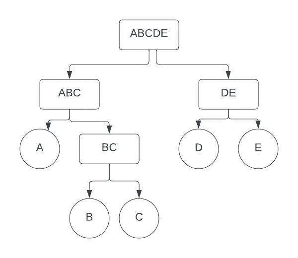
Finally, we assign unique codes for each letter: 0 for left and 1 for right. For instance, the code for D is 10. To reach D from the root, we move first to the right, then to the left. This system is efficient since we don’t need to denote when one code ends and the next begins — we simply stop whenever we reach a leaf. As a result, the most frequently appearing characters have the shortest codes:
A = 00
E = 11
D = 10
B = 010
C = 011
With this method, we can compress text quite effectively. Recall our earlier problem of distinguishing between backreferences and literals. Given the frequent recurrence of backreferences in the text, they would receive their own short, unique codes, thereby enhancing the compression efficiency. It’s important to note that while we’ve simplified the process here, the complete gzip algorithm is more complex.
Classification Through Compression
Now that we understand how compression works, we can go back to text classification. Consider three examples, x1, x2, and x3. x1 and x2 belong to the same category, while x3 falls into a different category. Let’s define C(·) as the compressed length of an object. The assumption we make is that C(x1x2) - C(x1) < C(x1x3) - C(x1). Here, C(x1x2) represents the compressed length of the concatenated x1 and x2. Essentially, C(x1x2) - C(x1) is the additional byte count required to encode x2 given the prior information of x1.
This idea forms the basis of a distance metric inspired by the Kolmogorov complexity — a theoretical measure defined as the length of the shortest binary program that can generate a string x. Due to the inherent uncomputability of the Kolmogorov complexity, a normalized, and computable alternative, the Normalized Compression Distance (NCD), is used instead. NCD uses the compressed length C(x) as an approximation for the Kolmogorov complexity K(x). Formally:
NCD(x, y) = [C(xy) - min{C(x), C(y)}] / max{C(x), C(y)}
The use of compressed length rests on the assumption that the length of x when maximally compressed by a compressor is approximately equal to K(x). For our purposes, gzip is used as the compressor. Consequently, C(x) denotes the length of x after gzip compression, while C(xy) represents the compressed length of x and y concatenated. With the distance matrix provided by NCD, we can apply k-nearest-neighbors for classification.
Let’s delve into how this is implemented in practice using Python. We can start with two text strings representing different categories, GroupA and GroupB, and a third string, StringUnknown, which we wish to classify. We compress each of these strings using gzip and calculate their respective lengths. Then, we concatenate StringUnknown with each group, compress the result and calculate their lengths.
Next, we compute the NCD for the unknown string and each group by subtracting the smallest compressed length of the group or the unknown string from the compressed length of the concatenated string, then dividing by the maximum compressed length of the group or the unknown string. This gives us a normalized measure of the “distance” of the unknown string from each group.
The group with the smallest NCD to the unknown string is considered the most likely group that the unknown string belongs to. In essence, the smaller the NCD, the greater the similarity between the unknown string and the group.
import gzip

GroupA = "This group is part of the business category. In these sentences we speak about profit, EBITDA and taxes."
GroupB = "Science category. In these sentences we speak about physics, chemistry, and other science related terms."
StringUnknown = "This is a sentence that we want to classify. It is a business sentence, we mention EBITDA, profit and taxes."

CompA = len(gzip.compress(bytes(GroupA, 'utf-8')))
CompB = len(gzip.compress(bytes(GroupB, 'utf-8')))
CompUnknown = len(gzip.compress(bytes(StringUnknown, 'utf-8')))
CompA_Unknown = len(gzip.compress(bytes(GroupA + StringUnknown, 'utf-8')))
CompB_Unknown = len(gzip.compress(bytes(GroupB + StringUnknown, 'utf-8')))

ncd_a = (CompA_Unknown - min(CompA, CompUnknown)) / max(CompA, CompUnknown)
ncd_b = (CompB_Unknown - min(CompB, CompUnknown)) / max(CompB, CompUnknown)

A_Diff = CompA_Unknown - CompA
B_Diff = CompB_Unknown - CompB

print("CompA: ", CompA)
print("CompB: ", CompB)
print("CompA_Unknown: ", CompA_Unknown)
print("CompB_Unknown: ", CompB_Unknown)
print("A_Diff: ", A_Diff)
print("B_Diff: ", B_Diff)
print()
print("NCD_A: ", ncd_a)
print("NCD_B: ", ncd_b)

if ncd_a < ncd_b:
    print("StringUnknown is in GroupA")
else:
    print("StringUnknown is in GroupB")
CompA: 110
CompB: 102
CompA_Unknown: 153
CompB_Unknown: 163
A_Diff: 43
B_Diff: 61
NCD_A: 0.42727272727272725
NCD_B: 0.5754716981132075
StringUnknown is in GroupAThis approach, using the NCD offers is just one method for computing the distance. However, other distance metrics can be employed.
The following method estimates the cross entropy between the probability distribution built on class c and the document d: Hc(d). The process involves the following steps:
- For each class
c, concatenate all samplesdcin the training set belonging toc. - Compress
dcas one long document to get the compressed lengthC(dc). - Concatenate the given test sample
duwithdcand compress to getC(dcdu). - The predicted class is
arg min C(dcdu) - C(dc).
In essence, this technique uses C(dcdu) - C(dc) as the distance metric, which is computationally more efficient than pairwise distance matrix computation on small datasets. However, it has some drawbacks. Most compressors, including gzip (as mentioned above), have a limited “window” they can use to search back through the repeated string or keep a record of. As a result, even with numerous training samples, the compressor may not fully exploit them. Additionally, compressing dcdu can be slow for large dc, a problem not solved by parallelization. These limitations prevent this method from being applicable to extremely large datasets. As such, the NCD-based approach presented above, which avoids these limitations, becomes particularly appealing for text classification tasks on large datasets.
Downsides and Drawbacks
Despite the ingenuity of applying compression algorithms for text classification, the approach is not without its limitations. The size of the lookback window of the LZ77 algorithm, for instance, presents a potential drawback. This algorithm searches the prior text to find matches, but its effectiveness can diminish when dealing with very long text.
In addition, the method does not grasp the subtleties of language, such as synonyms or context-specific meanings. The absence of this linguistic sophistication may hinder its performance on tasks requiring a deeper understanding of language nuances. Furthermore, the computational intensity of this approach can escalate rapidly when dealing with larger datasets, given the O(n^2) complexity of K-Nearest Neighbors (KNN).
Lastly, some controversy surrounds the code and results of the original paper that introduced this method. Some of the datasets used seem to have issues, though not due to the authors’ mistakes. Additionally, there has been some debate regarding how the results have been scored. For a detailed look at these issues, you can check out this blog post and follow the discussion on GitHub.
Conclusion
This is a really interesting approach, and while it may not be perfect, it provides much food for thought.
To get hands-on with the concepts discussed in this blog, you can check out this repository that I made. It provides a simple implementation of LZ77 and Huffman encoding, allowing you to experiment with these algorithms and see how they work in practice.
For a more in-depth understanding of gzip, consider reading this blog post. This article offers an excellent explanation of the LZ77 algorithm. Of course, you should read the original paper, available here, which is very well written and understandable.
← Back to all posts